Power Query - Working with columns

When you are working with Power Query you often add, remove and modifying columns in your queries. There are tons of ways to do that, in this part we look on the most common cases.

Before you read on, make sure you have completed the previous part Power Query - Get started in Excel because we continue working with the data we created there.

Combining data into a new column

In the panel Queries & Connections double click on Player to open the Power Query editor again.

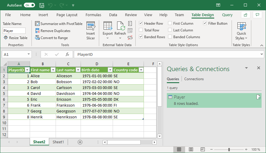
Now the Power Query editor should look something like this:

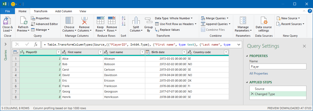
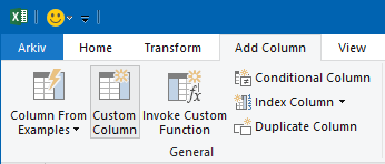
In the data we have first and last name in two separate columns. The first thing we will do is to make a new column where we see both these names. Click on Add Column > Custom column.

Now you get a new window looking like this:

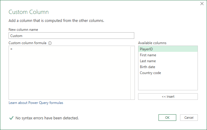
In this window you give the new column a new and enter a formula. Enter the following formula:

Formula

[First name] & " " & [Country code]

Yes, we are intentionally making a mistake by adding first name with the country. We will fix that in a moment. Change New column name to Name. The window should now look like this:

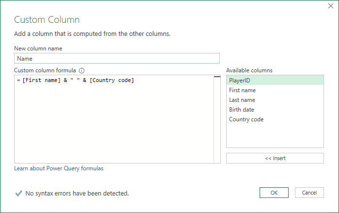
If it does, click OK. The Power Query editor now looks like this:

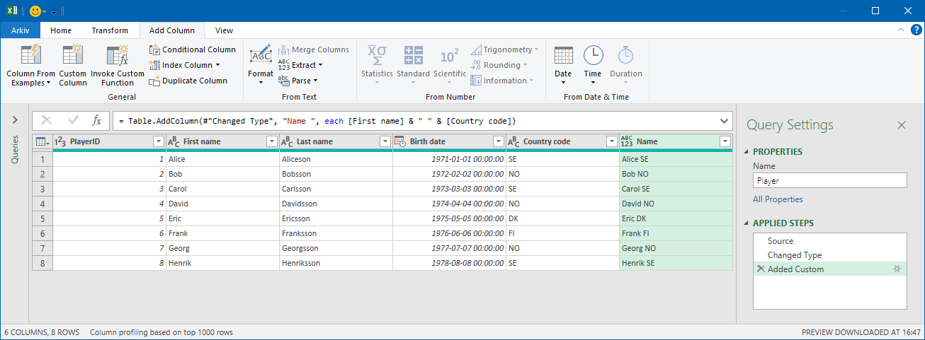
Note that you now see a new column called Name. Also note that in Applied steps a new row has been added.

Removing columns

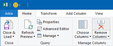
We are still pretending that we have not noticed our previous mistake. We do not want to keep the columns First name and Last name. Therefore, select the column you want to remove, click on the Home > Remove columns.

Now the editor should look like this:

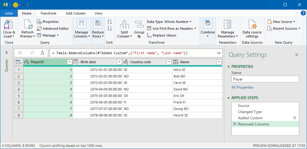
As you remember we used the First name column in our formula that we created earlier. If this was an ordinary Excel formula the Name column should now be broken. But in Power Query formulas works in a different way. Have a look on Applied steps:

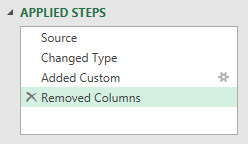
This is giving us a quick overview on which steps we have taken to create the query. There are four steps:

• Source – We are getting data from the Excel table
• Change Type – We specify the data type for every column
• Added Customer – We added the Name column
• Removed Columns – We removed the two old name columns.

The first two steps we got for free when we created our query in the previous tutorial. The other two steps we just created.

If you click on any of these steps, you see how the data looks like after that step has been applied. Click on Added custom and Removed columns to see the difference.

Changing a previous step

As you might have noticed it is possible to edit each step. In the Applied steps panel, double click on Added custom. Now we get back this window:

Fix our incorrect formula by replacing [Country code] with [Last name] and then select OK. Now you should see this:

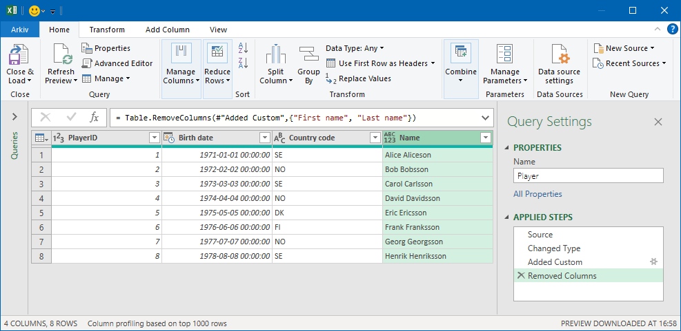
If you in Applied steps double click on Remove Columns nothing will happen. That is because there is no explicit editor for removing columns. But instead, you could edit this formula that you see in the Power Query editor:

Formula

= Table.RemoveColumns(#"Added Custom",{"First name", "Last name"})

This formula specifies that First name and Last name should be removed. You could edit this formula manually if you want to. You could also remove steps in Applied steps panel.

Advanced editor

Click on Home > Advanced Editor.

Then you will see this:

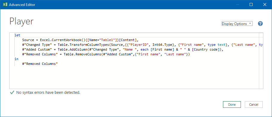
This is showing the same information that you see in Applied steps but in more detail. This is what the editor says:

• Line 2: Create a table named Source from a table in the current file.
• Line 3: Create a new table named Changed type, based on the table Source by specifying data type on each column.
• Line 4: Create a new table named Added custom based on the table Change type by adding a new column.
• Line 5: Create a new table named Removed Columns based on the table Added custom by removing columns.
• Line 7: Use the table Removed Columns as the output from the query.

In most cases you never need to use the advanced editor, but it is good to know that it exists. We will not make any changes here so close the editor.

Data types

In the Power Query editor, you now should have four columns:

In each column one data type per column could be used. One column could for instance contain whole numbers, another column could contain dates and a third could contain text. This is different from spread sheets where you specify the data type on every individual cell.

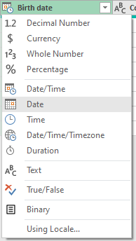
If you look on the Birth date column you see that every cell contains a date and a time. This because the data type is set to Date/Time. Change the data type by clicking on the icon just left to the column title and change data type to Date.

Now the editor should look like this:

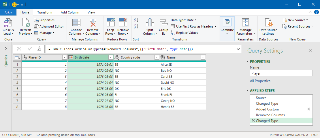
That is a bit better. If you select a column you see which data type they are using in Home > Data type.

Check which data types the other columns are using.

Now we have the birth date in a pretty way in our table. But wouldn’t it be nice to show the age of each player too?

Working with dates

While you have the Birth date selected, click on Add column, select Date and then in the menu select Age.

Now a new column will be added to the editor:

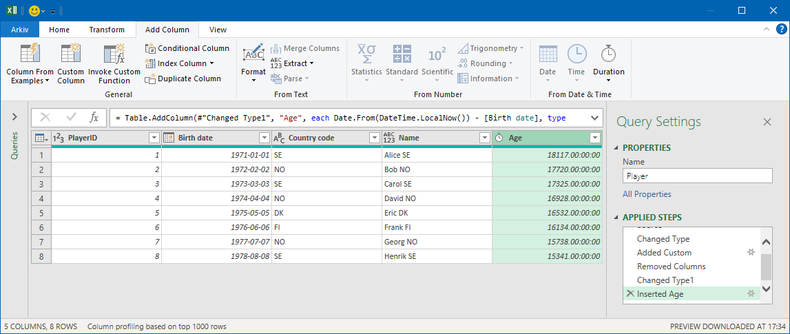
The Age column has the data type Duration and it shows the age in days, hours, minutes, and seconds. This is great for computers, but humans prefer to calculate age in years, so we need to fix that.

Select the Age column, click on Add column > Duration and select Total years.

Now a new column appears showing Total Years:

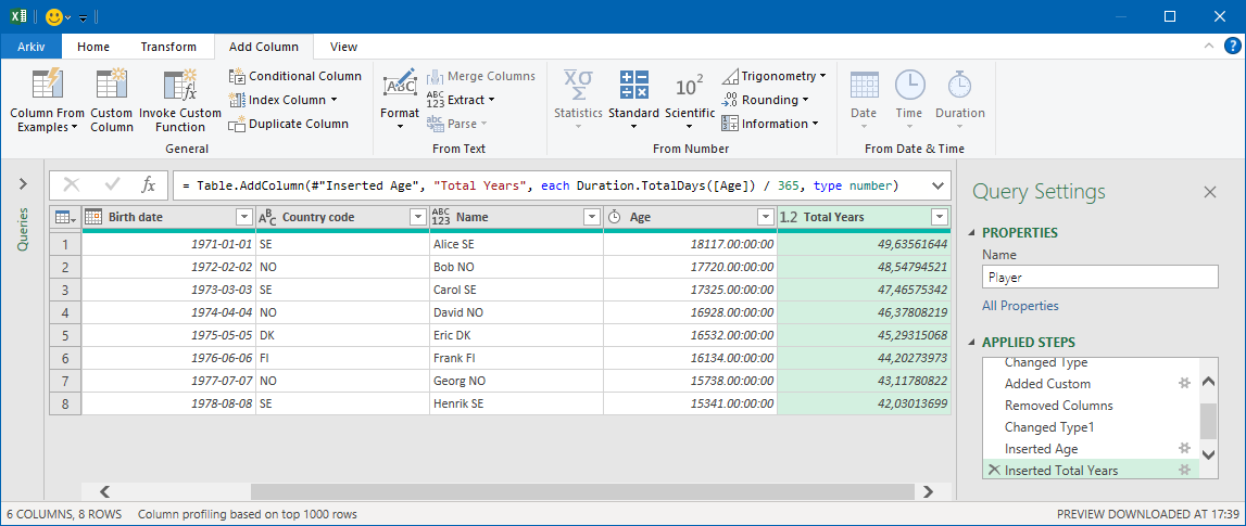
The Total Years column is calculated by dividing the Age column with 365. So, this does not take leap years in account which might be a problem. But to keep this tutorial simple we will ignore that.

Now we have the age in years, but it is shown as a decimal number. Showing this as a whole number is preferable. Changing the datatype to Whole number might seem to be a good idea, but then the ages might be rounded incorrectly. Instead we will specify how they should be rounded. To do this, click on Transform, Rounding and select Round down.

Now the editor should look like this:

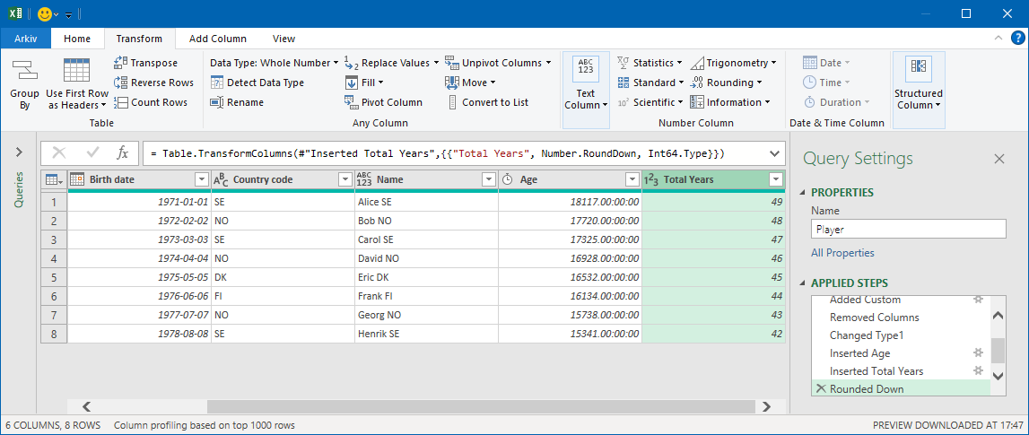
This is a lot better. Now, have a look on the Applied steps panel. On every task you did you see a new step in there. You could also edit some of these steps. For instance, in the step Inserted age click on the settings icon. Now the Custom column editor will show the formula that was used when you selected to insert age. You do not need to change this, so just close this window.

Every time you decide to add, remove, or transform a column in the tool bar a formula will be created that you later could edit in the Applied steps panel. Remember that you call see all details in the Advanced editor.

Now we will end this by doing some minor clean ups. Make sure you have selected the last step in the Applied steps panel. Start by removing the Birth date and the Age columns.

Then, right click on the Total years column and select Rename. Name the column Age. Now the editor will look like this:

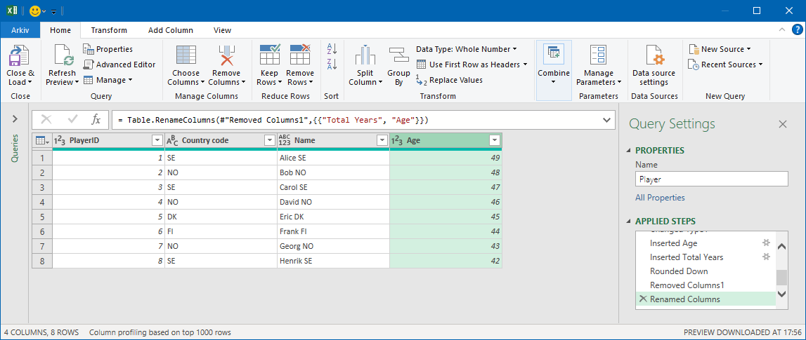
Click on Home > Close & Load. Now you should be back in ordinary Excel and you should see this:

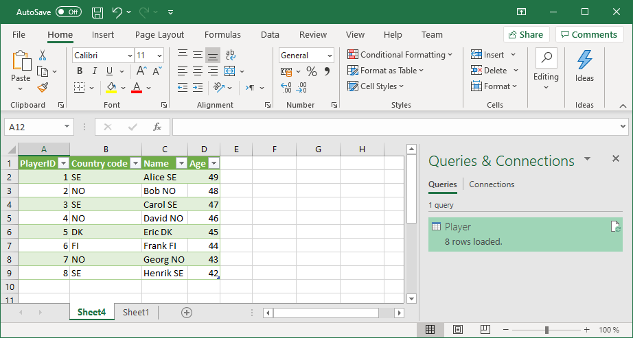
If you go to Sheet1 and change a name and a birth date on a player, and then refresh the query you should see these changes in this view.

Summary

You can check the final result of this part in this file: power-query-part-2.xlsx.

In this tutorial learned how to add, remove, and modify columns and how to use the Applied steps panel. In many cases when you will add a column you will find a short cut in the toolbar that does what you want.

When you have been adding column, you have always based those on the data you already have in your table. But you could also add columns from other queries, when look on that in the next part: Power Query - Joining data.