Power Query - Grouping and filtering data

When you are working with data you often want to do some kind of summarizing. With Power Query you do this with grouping. Just like join, this is similar how it works in SQL.

Before you read on, make sure you have completed the previous part Power Query - Joining data because we continue working with the data we created there.

Referencing previous queries

Now we will create some statistics for each country. We want to know the number of players from each country, and what the average age is.

The first thing we need to do is to decide which data source we want to use. In your Queries & Connections panel you have three queries. The query PlayerCountry would be a good starting point for us. But we do not want to modify this query because it is useful as it is. Another option would be to copy that query. But the option we will use is to make a reference. Right click on PlayerCountry and select Reference.

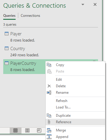
When we are doing this, we use the result from the PlayerCountry query as the data source. This means that if we a making changes to PlayerCountry this will also affect our new query. You should now see the Power Query editor:

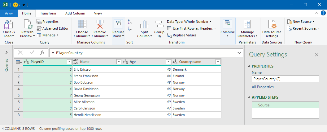
The data you see is identical to PlayerCountry.

Grouping data

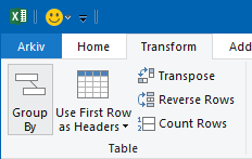
Now we will start to group the data. Select Transform and then click on Group by.

Now you are being asked how to group the data. Configure the settings like this:

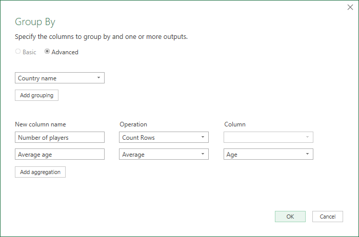
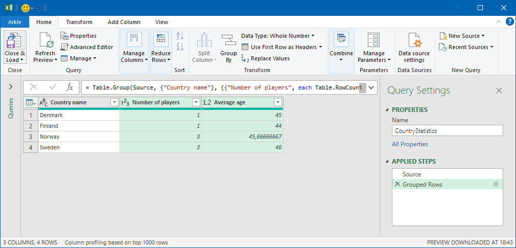
When data is grouped, all rows that have the same content in the columns you have selected will be in one single row. Then you could do aggregations on the other columns. In our case all rows where column Country name is identical will be grouped. Then for each of these groups we will get the number of players and the average age on the players. Now, click on OK.

Now you see the result in the Power Query editor. Give the query the name CountryStatistics and then click on Home > Close & Load.

Now you see the result in Excel:

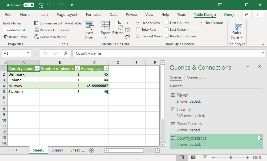
Grouping is quite easy to do. If you want to challenge yourself, try changing the query so that you see:

• The age of the youngest player of each country.
• The age of the oldest player of each country.
• The average age with one decimal. You need apply rounding as an additional step.

Analyzing Rock-Scissor-Paper data

The players we have been used is obsessed rock-scissor-paper players. It is said that every year when the earth is furthers away from the sun the get together at midnight and play an intense tournament. Every player plays against every other player twice, once as a home-player and once as an away-player. The log every move they make. Our job is to figure out which player are the winner or the tournament.

Start by downloading this file: rock-scissor-paper.txt.

If you open the file you see start it starts like this:

Advanced editor

GameID*HomePlayerID*AwayPlayerID*HomeMove*AwayMove
1*1*8*P*S
1*1*8*S*P
1*1*8*P*R
1*1*8*R*R
1*1*8*S*S
1*1*8*P*P

This is a crazy file format! But as you could guess every row contains of:

• Game ID (just a number)
• ID of the home player
• ID of the away player
• Move of the home player. That is, Rock, Scissor or Paper
• Move of the away player.

As you could guess we will have to do a lot of fun stuff to figure out which player that are the tournament champion :-)

Reading and parsing the file

In Excel, select Data and then From Text/CSV

When you have selected the file, you will see this:

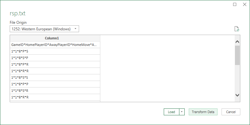
If this had been a CSV-file then Power Query would have been able to parse that correctly and you would have seen all columns directly. But with this we do not have that luxury. But it is not too hard to fix. Click on the button Transform Data.

Now you are in the Power Query Editor. You see all data in one single column. The first thing we will do is to separate this into several columns. Select Transform > Split Column > By Delimiter.

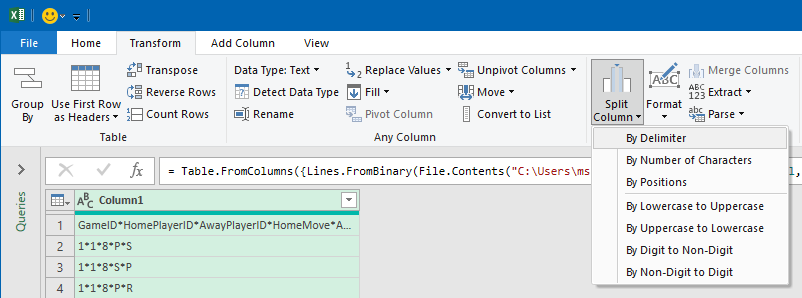
Now you are being ask which delimiter to use. Select asterisk (*) as below and click OK.

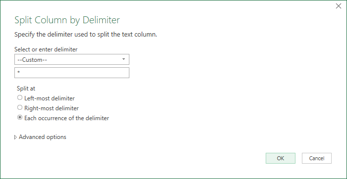
Now you see the data in five columns, much better! The only problem now is that headers are offset. Fix that by selecting Transform > Use First Row as Header.

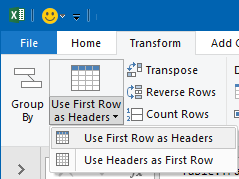
Now you see the data as this:

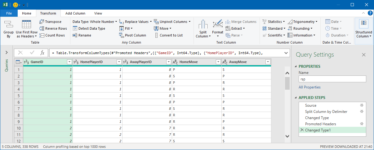
In just two steps we converted this file into a table we could use.

Creating column from example

In this version of Rock-Scissor-Paper a player will get 1 score of if the player picks:

• Paper and the opponent Rock
• Rock and the opponent Scissor
• Scissor and the opponent Paper.

Otherwise it will score 0. The first player to reach 3 wins the game.

We will use conditions to solve this which we have not used before. But conditions could only operate on a single column so we will create a new column based on the two moves-columns.

We could do this by adding a Custom column and write the formula manually. But this time we will instead let the editor guess the formula to us. Select Add column > Column from Examples.

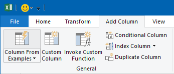
Now we are being asked to write examples:

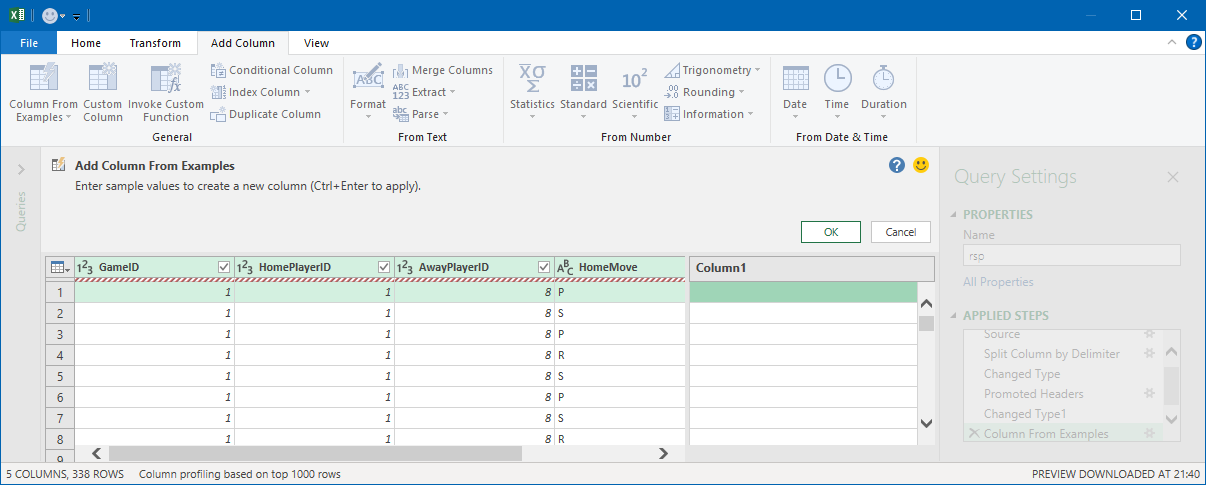
In the first row HomeMove is P, and AwayMove is S. We want there that the text P-S in the new column, so we just enter that the example on the first row and press enter:

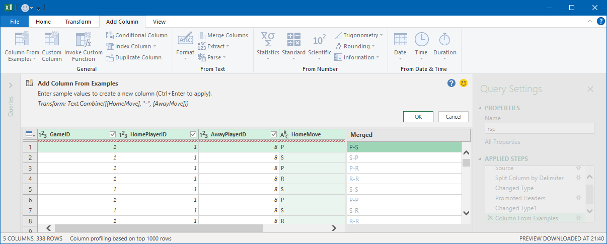
As you see the editor now guesses that we want to use the formula:

Formula generated from examples

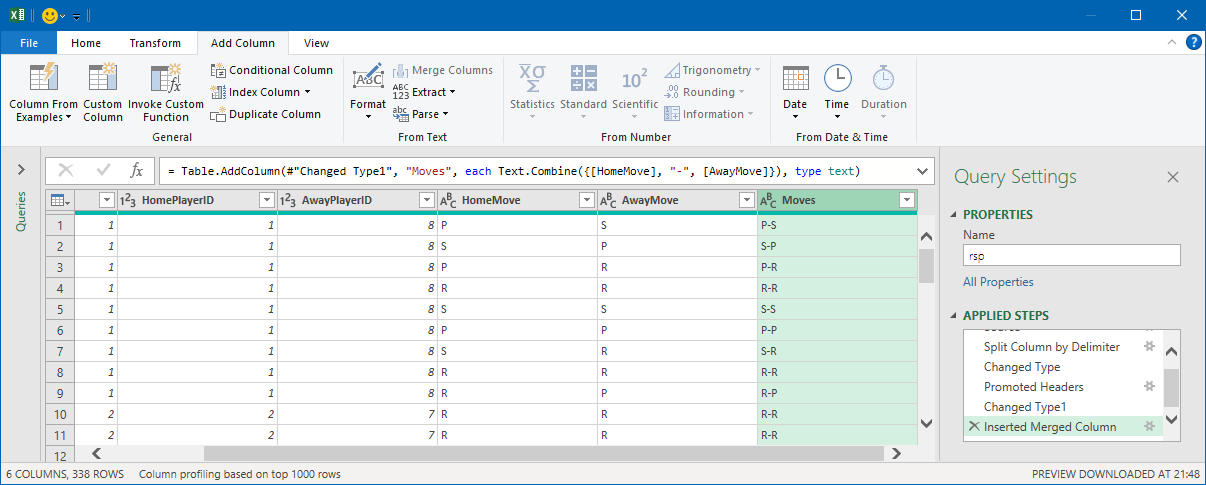
Text.Combine({[HomeMove], "-", [AwayMove]})

And this exactly what we wanted to use! If the formula is incorrect you could enter more examples and, in many times, you will get the right formula. This feature is amazing and will in many cases save you from writing complicated formulas. Rename the new column to Moves and then click on OK.

Getting the score

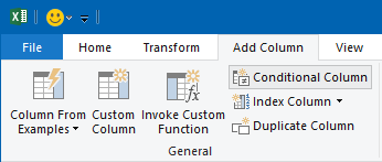
The next step is to create a column where we see the score the Home-player. Click on Add Column > Conditional Column.

Now we will setup the conditions where the Home-players gets one score. That is if:

• Home plays P and away plays R.
• Home plays R and away plays S.
• Home plays S and away plays P.

Otherwise the score will be 0. Setup the conditions like this:

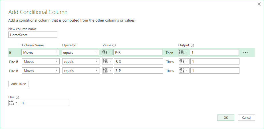
Also set the column name to HomeScore and click OK. Now in the editor you see this:

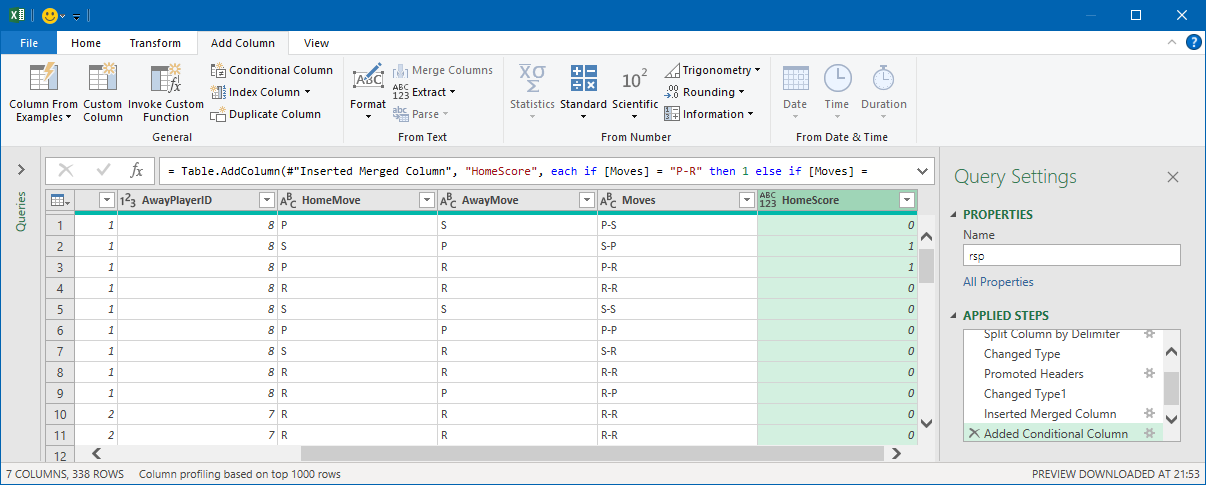
Now you see the rows where the home player gets the score.

Next, we setup the score for the other play. Again, click on Add column > Conditional Column.

You could setup the conditions similar like we did before, that totally works. But instead we use a bit of different logic. The away player will not get a score if:

• The home user got a score.
• The players made the same move.

Otherwise it will score 1. Setup the conditions like this:

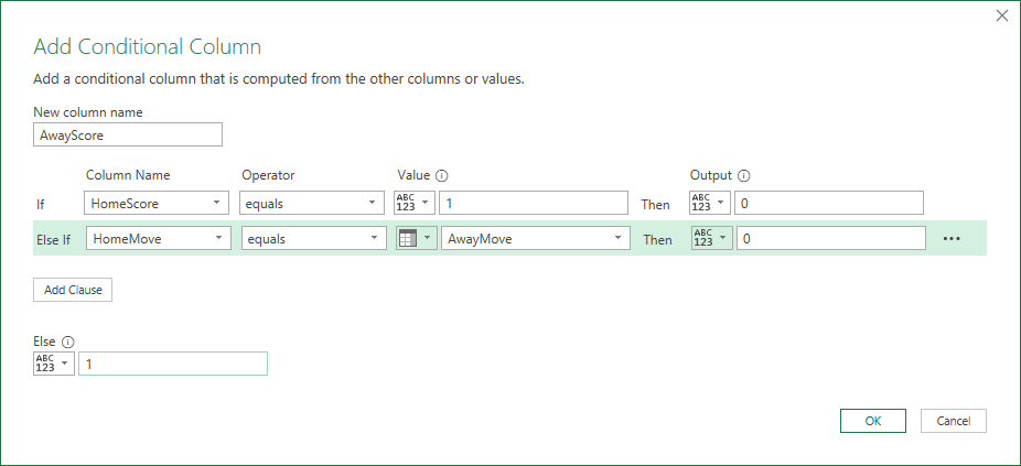
Set the name to AwayScore and then click OK.

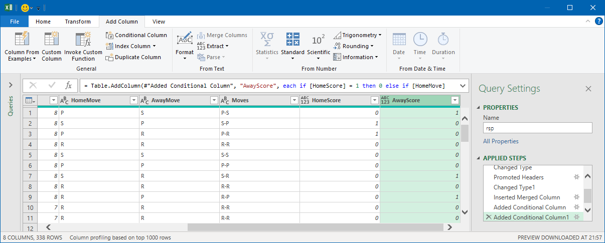
Now we see the score each player gets after each move.

Summarizing the score

Instead of seeing game score for each round, we want to see the total score after each game. We solve this with grouping. Select Transform > Group By.

Group by GameID , HomePlayerID and AwayPlayerID and the sum up the HomeScore and AwayScore.

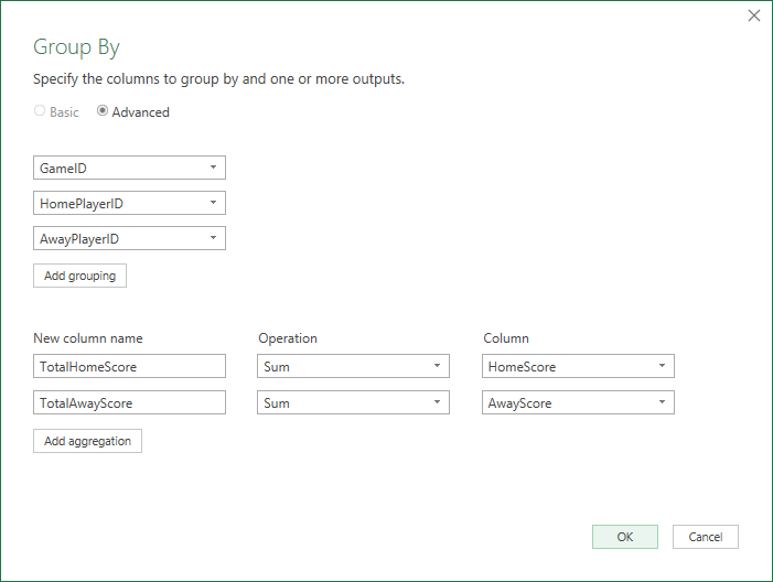
Then press OK and you see this:

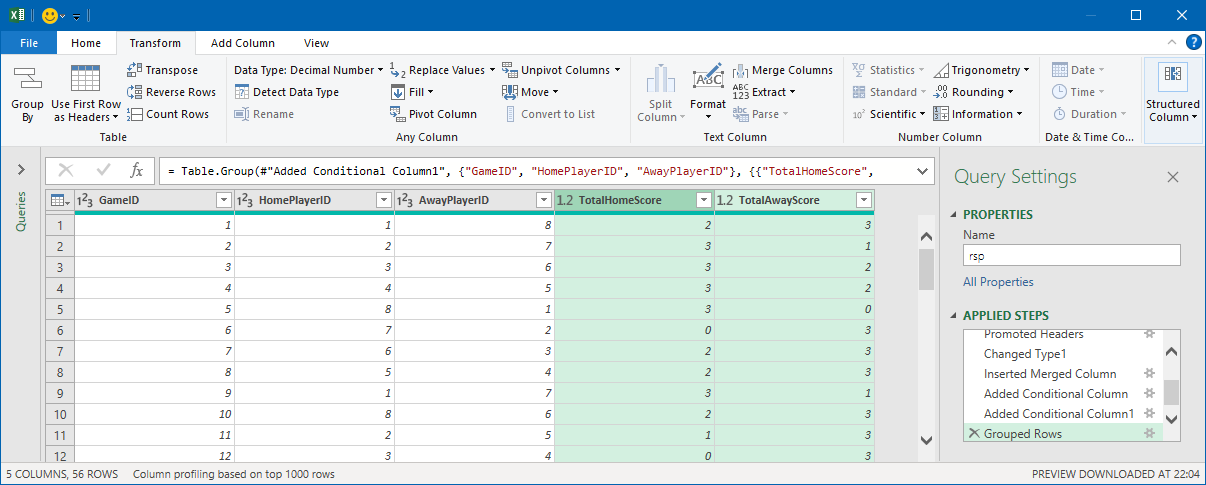
As you see each game one player has the score 3 which is just what we expected.

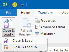
Now are done with this query. Name of GameScore and the and select Home, Close & Load and then Close & Load To….

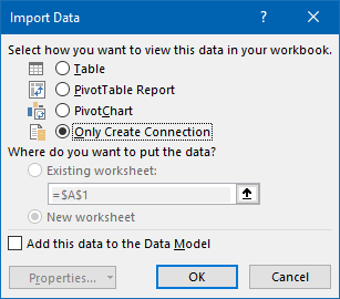
This query will just be used as base for other queries, so we do not need to see it in Excel. Therefore, select Only Create Connection and press OK.

Getting the winners

Next problem to solve is to get the winner of each game. The best way to do this is to add a new conditional column in the GameScore query, comparing the TotalHomeScore with TotalAwayScore and then user HomePlayerID or AwayPlayerID depending on the conditions. But we will not learn much form that and will select a different approach.

Instead we will create two separate lists. One list where the home player is the winner, and another list where the away play is the winner. And then we merge these two lists.

In the Queries & Connections panel, right click on GameScore and select Reference.

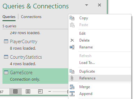
Now you see the editor with the data referenced from GameScore. As mentioned earlier, a player wins a game if it reaches the score 3. We will now filter out each game where the TotalHomeScore has the value 3. In the TotalHomeScore column, click on the drop-down button and select the filter like this:

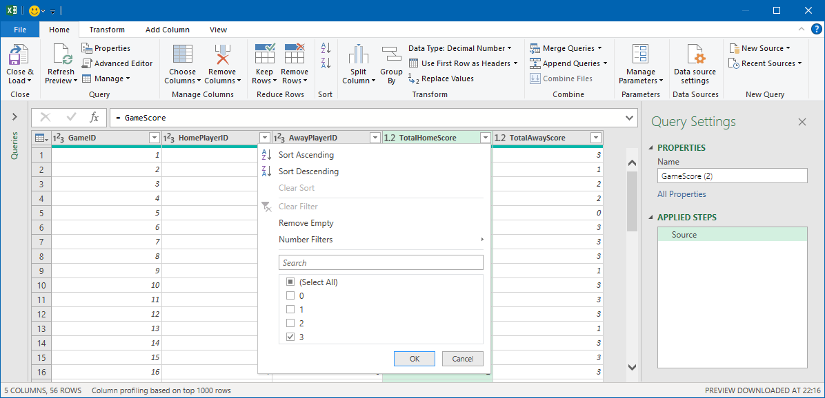
After the filter has been applied, we just want to keep the HomePlayerID. Right click on the column and select Remove Other Columns.

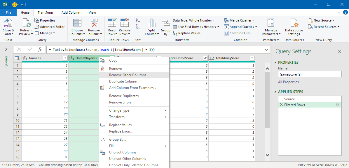
Rename the column to WinnerPlayerID and name the query HomeWinners.

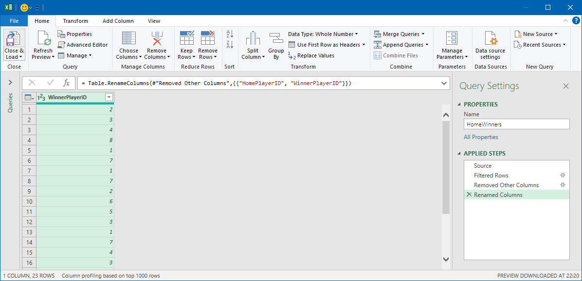
Now we are done with this query. Finish it by click Home > Close & Load. And as before you do not need to show this query in Excel.

Now repeat this but filter out the away winners instead. Name that query to AwayWinners. Remember to name the column WinnerPlayerID.

Combining the winners

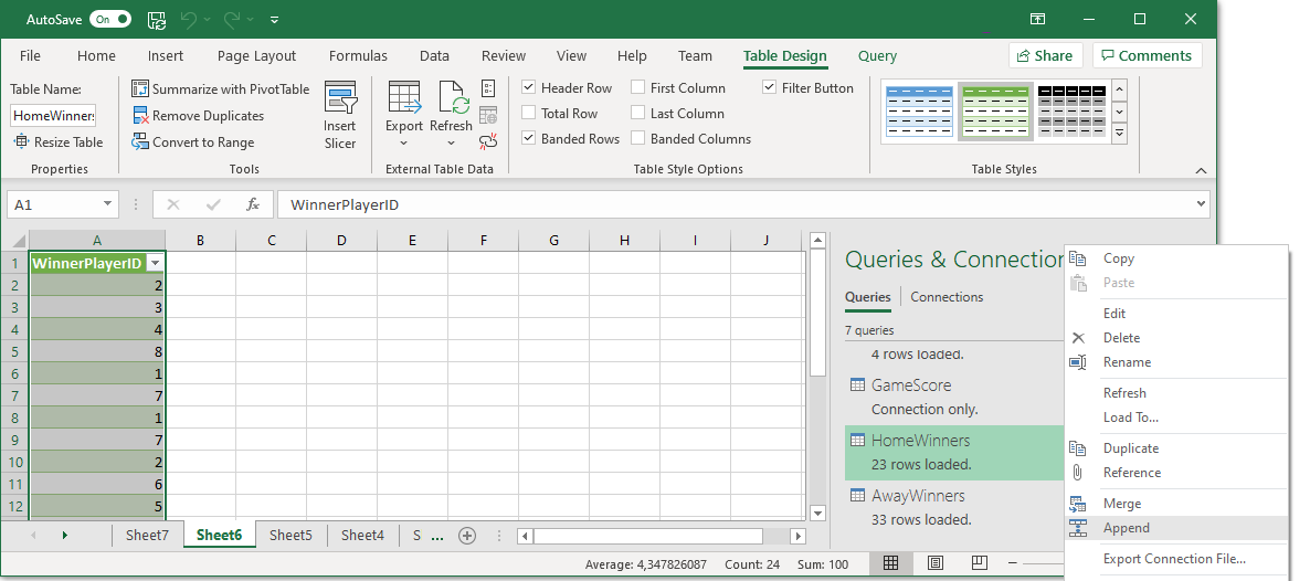
In the Queries & Connections should now you see the HomeWinners and AwayWinners. Now will combine these two lists into a single list. Right click on HomeWinners and select Append.

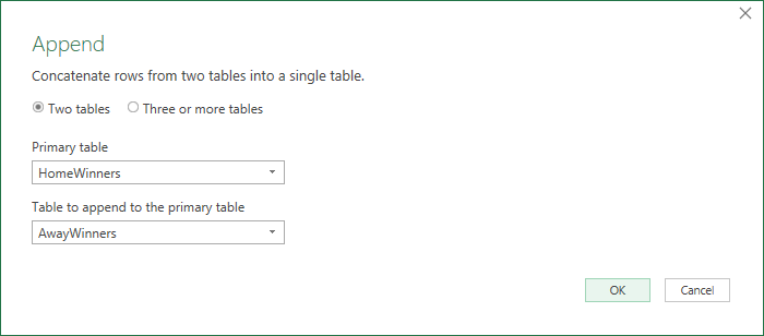
Select HomeWinners and AwayWinners and then click OK.

When you click OK you will see the winner of every game. If you have done everything correctly you should have 56 rows with a single column. If the tables would have more columns you would see these two.

Getting number of victories for each player

Now we just want to get how many times each player has won. Select Transform and then Group By.

We group by WinnerPlayerID. Then we just count the number of rows for each player and call that column Victories.

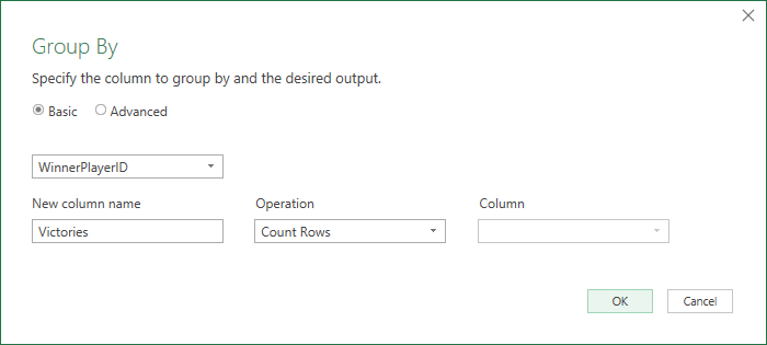
Now you should see the result in the editor.

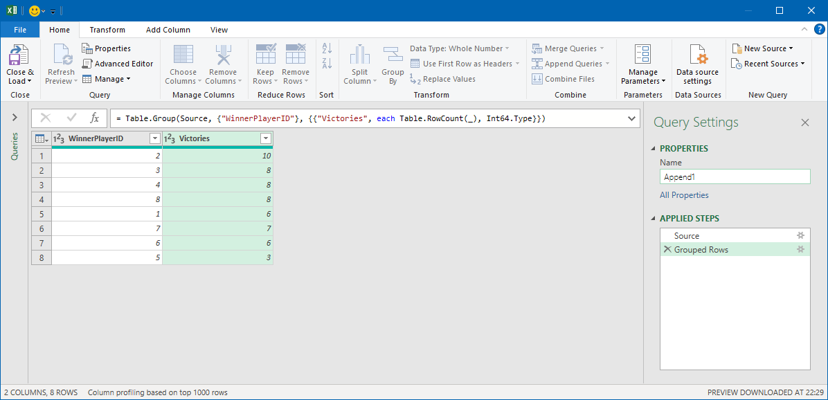
You could sort the list by Victories by clicking on the drop-down button and select Sort Descending. As you see player 2 has 10 victories, while player 5 just had three.

Call the query WinCount and close the editor by selecting Home, Close and Load. Add the result to an Excel spreadsheet if you want to.

Of course, it would be nicer to see the name of the player instead of just the id. As a final challenge, you could try to solve this by merging PlayerCountry with then new WinCount query.

Summary

You can check the final result of this part in this file: power-query-part-4.xlsx.

In this part we parsed data from a strangely formatted file, and then used some logic to figure out the score of each player and then we summarized everything.

I hope you understood most part of this. I also hope that you know what you could do with Power Query. I think it is a very powerful tool and I used it often when I am analyzing data.

In all four part tutorial we have touched the most important features in Power Query. Obviously, there is a lot more. But the things you have learned from this should cover a lot, and you are most likely you find more features on your own.