Power Query - Joining data

Sometime useful to combine data from two tables when you are working with Excel. You could do this with functions like VLOOKUP. It works, but it is a pain to use. If you instead are using Power Query, you could easily join data from two tables. If you know SQL, you will find this familiar.

Before you read on, make sure you have completed the previous part Power Query - Working with columns because we continue working with the data we created there.

Getting data from Wikipedia

The data we have now is just a single table player names, country codes and some other data. In this part we will add a new column so we could see the name of the country instead of the country code.

But before we do this, we need a data source where we see with the country code and country name. For our existing data we use an Excel table as a data source. This time we will instead use a Wikipedia-page!

In Excel, select Data and then From Web.

Insert the following URL:

https://en.wikipedia.org/wiki/ISO_3166-1_alpha-2

Then click OK.

Now all tables from the page will be loaded and you will be asked to select the table you want to use. Select the table Officially assigned code elements. Before we use the data, we want to make some modifications. Therefore, click on Transform data (if you select Load the table will be loaded into Excel as it is).

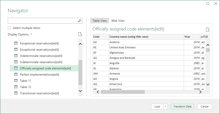
Already it looks pretty good! But there are some data we do not need.

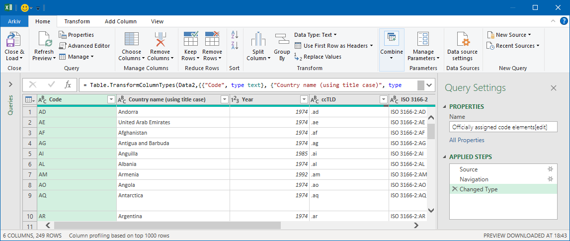
First, remove all columns except for the first two.

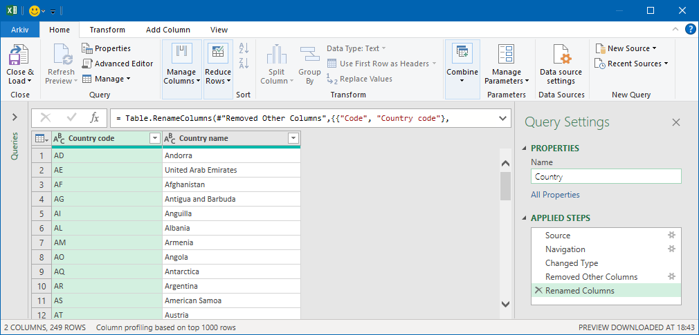
Then rename the first column to Country code.

And then rename the second column to Country name.

If you want to cheat, open the Advanced editor and replace the content with this code:

Advanced editor

let
    Source = Web.Page(Web.Contents("https://en.wikipedia.org/wiki/ISO_3166-1_alpha-2")),
    Data2 = Source{2}[Data],
    #"Changed Type" = Table.TransformColumnTypes(Data2,{ {"Code", type text}, {"Country name (using title case)", type text}, {"Year", Int64.Type}, {"ccTLD", type text}, {"ISO 3166-2", type text}, {"Notes", type text}}),
    #"Removed Other Columns" = Table.SelectColumns(#"Changed Type",{"Code", "Country name (using title case)"}),
    #"Renamed Columns" = Table.RenameColumns(#"Removed Other Columns",{ {"Code", "Country code"}, {"Country name (using title case)", "Country name"}})
in
    #"Renamed Columns"

In the query settings, change the name to Country. If you have done everything correctly, you should see this:

Click on Home > Close & Load and you should now see the table in Excel.

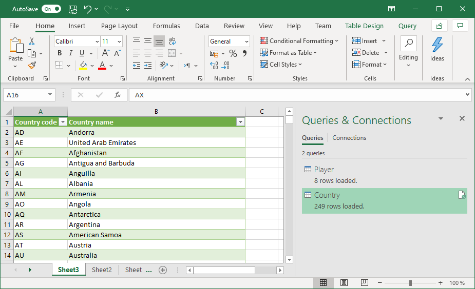
Every time you select to refresh the data; Excel will go to Wikipedia and fetch all new countries from that page. Pretty cool, I think.

Joining data

In the Queries & Connections panel you now have two queries. Now we will combine these two. Right click on Player and select Merge.

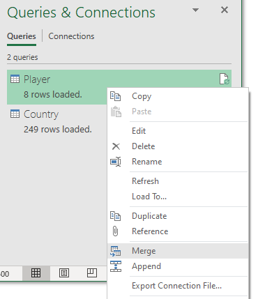
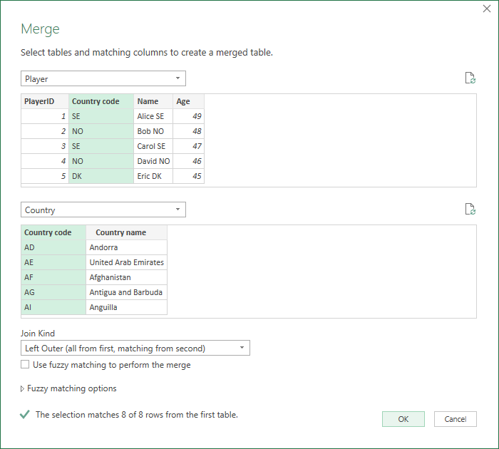
Now you will see a new window where you select which tables you want to merge. You should also select on which columns which the data will be joined. We are just using the column named Country code in each table, but it is possible to join data on multiple columns.

You should also select how the data should be joined with the Join Kind setting. This time we use Left Outer. Make sure you have setup this like the image below and then click OK.

Now the Power Query editor look like this:

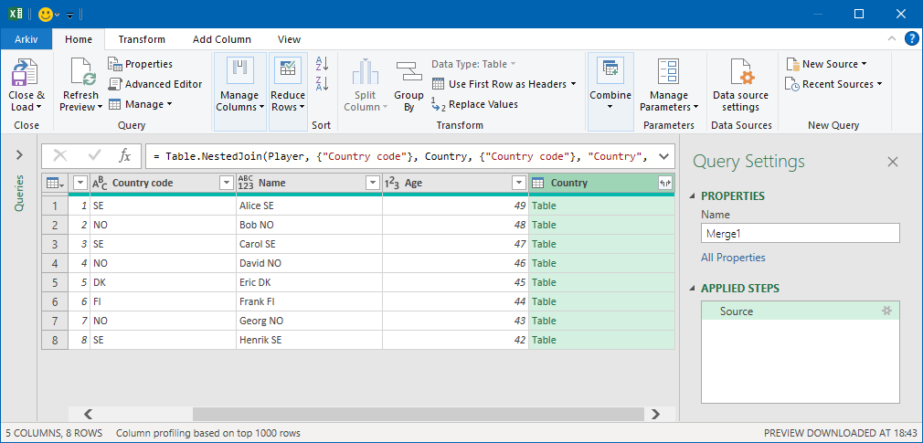
As you see you have all the columns from the Players table. But you also have a new column named Country. In this column you have all the matching rows from the Country table. To make this more useful, click on the expand button and select that you only want to see the Country name column.

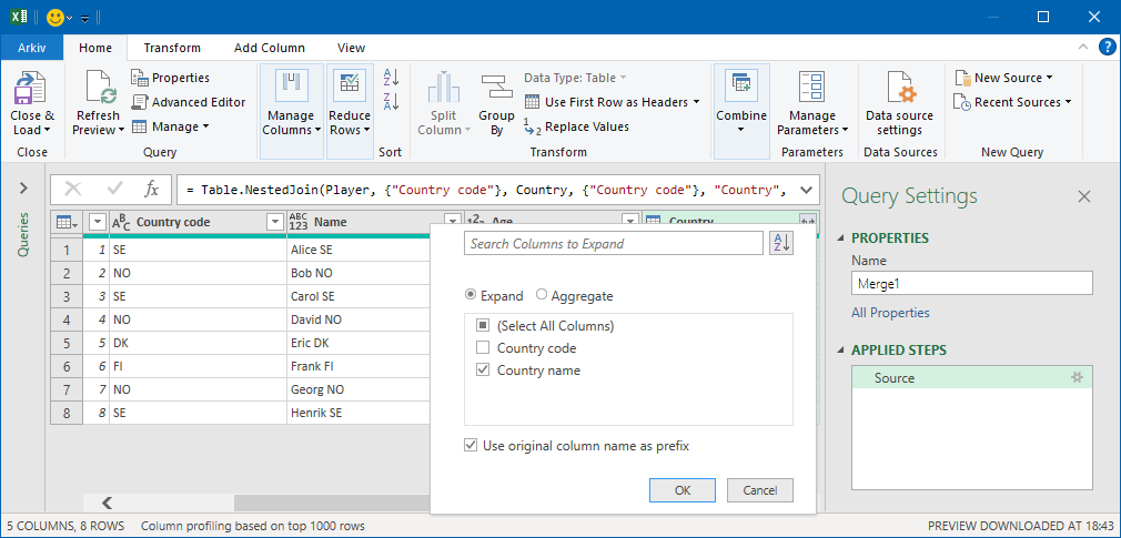
After you have clicked OK you will see the name of the country of each player in a new column. Rename this column to Country name. Also remove the column Country code. And then change the name of this query to PlayerCountry.

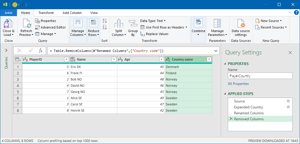
Then select Home > Close & Load to see the data in Excel.

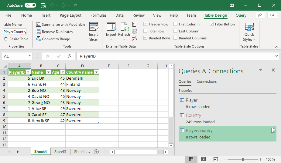
Well done! As you see you now have a third query in the Queries & Connections panel.

Now you could do some experiments. Go to Sheet1 were you have your original data. Change the country code of a person. Then select Data and then Refresh all.

After a few seconds you will see the new country name on the person you changed. Remember that when you pressed that button, data was fetched and analyzed from Wikipedia and combined with the data that you have in spreadsheet.

Summary

You can check the final result of this part in this file: power-query-part-3.xlsx.

In this tutorial we fetched data from Wikipedia and merged it local data. After this I hope you see the power with Power Query. Obviously, you could get data from other data sources, like a real SQL database or some external Excel file. Just click on Data > Get Data to see which options are available.

But this is not all! There is one other major concept left we will look into the next part: Power Query - Grouping and filtering data.